Microsoft Excel: Secrets of Effective Non-Visual Work with Tables.

05 Jul, 2024

written by

Part 2 About Ranges and Tables in MS Excel

It’s important to understand that although the workspace of an Excel sheet is a grid that resembles one large table, it doesn’t limit us in creating tables. The workspace allows for placing several different tables on one sheet, as well as individual cells not related to any table.

A table on a sheet is an area of filled cells without any empty rows or columns. Two tables on one sheet must be separated by one or more empty rows or columns. The terms “table,” “cell range,” and “data area” in Excel are synonymous and have the same meaning.

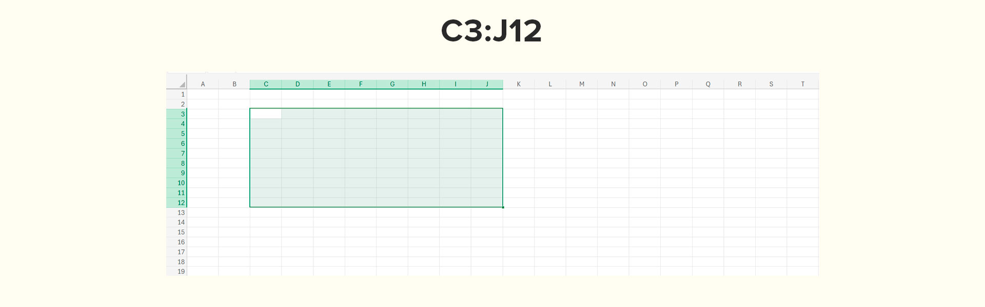
The notation for cell range coordinates is as follows:

For a linear range (one row or column): “A1:A5” for cells from “A1” to “A5”.
For a rectangular range (rectangular area): “A1:B2” for the cells “A1”, “A2”, “B1”, and “B2”.

Keyboard Commands for Selecting a Range

In Microsoft Excel, there are several keyboard commands for selecting a range of cells. Here are the combinations used for selecting linear ranges:

“Shift + Up or Down arrow” – selects cells in one column;
“Shift + Left or Right arrow” – selects cells in one row;
“Ctrl + Shift + Up or Down arrow” – selects from the active cell to the beginning or end of the column;
“Ctrl + Shift + left or right arrow” – selection from the active cell to the beginning or end of the line;
“Ctrl + Space” – selects all cells of the current column;
“Shift + Space” – selects all cells of the current row;
“Ctrl + Shift + 8” – selects a range of cells around the active cell (number 8 in the numeric row);
“Ctrl + A” – selects the contents of the entire sheet;
First, “End”, then “Shift + arrow up, down, left, right” – selection from the current location to the end of the active area.

To select continuous rectangular areas, first select a linear range in a row, then in a column. You can also select a linear range in a column first, then in a row.

When selecting a range, screen readers will announce the coordinates of the top-left and bottom-right cells of the selected range. To listen again to the information about the coordinates or content of the range, use keyboard commands to obtain information about the content and coordinates of the cell.

Managing Table Structure

In Microsoft Excel, “Managing Table Structure” refers to the ability to change the format, size, as well as add or delete rows and columns in a spreadsheet.

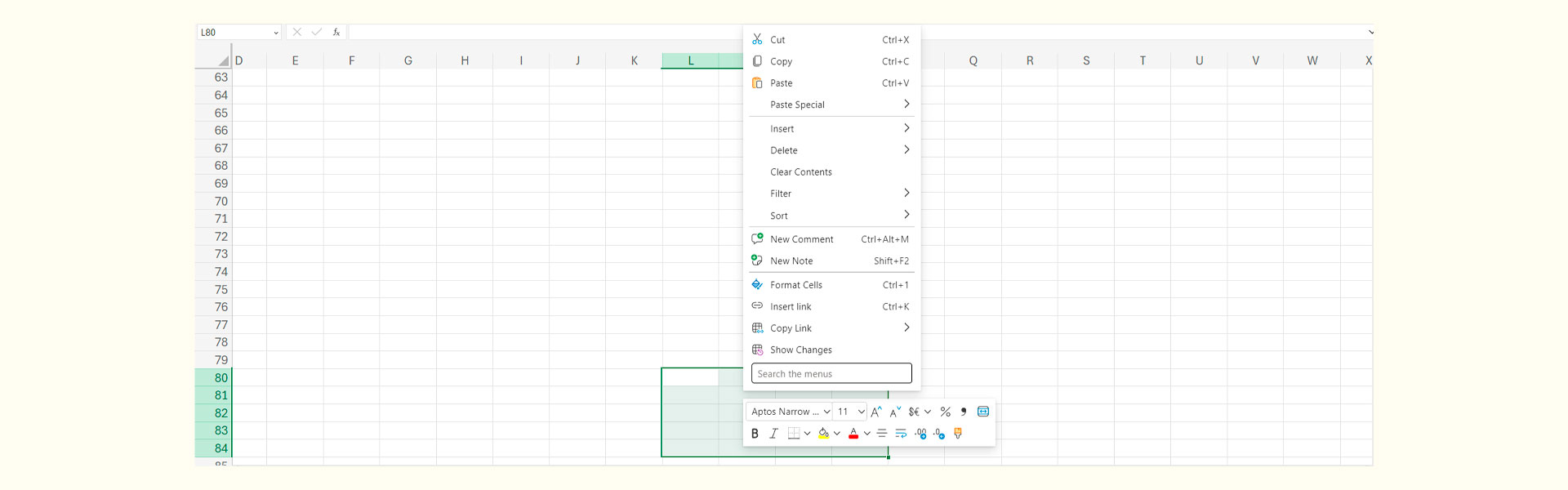
Adding new cells, rows, or columns is necessary for expanding the table and is quite common in work. For this, you can use the “Insert” command from the context menu by pressing “Shift + F10” or “Ctrl + Shift + =”, or “Ctrl + +” (plus) on a selected cell. All three combinations will bring up the insertion window, where you need to choose the insert element and click “Ok”. Note that this action will shift all data to the right or down from the selected cell.

Deletion works in a similar way. To do this, you need to select the cell you want to delete or that is in the row or column being deleted, and bring up the deletion window by pressing “Shift + -” (minus) or “Shift + F10” and selecting “Delete”. When deleting, the shift will be to the left or up, depending on which element is being removed. Additionally, you can use the commands in the “Cells” group on the “Home” tab. After inserting new rows or columns, Excel will automatically recalculate formulas and update related data.

It’s important to remember that proper management of table structure facilitates more convenient data analysis and increases work efficiency with the program.

Cell Formatting

Previously, we mentioned that Excel cells can contain a variety of information, including text, numbers, dates, formulas, hyperlinks, and other data. Due to the extensive list of data types that can be contained in cells, MS Excel has a specialized parameter – “Cell Format”. This parameter is added to provide the ability to more flexibly and accurately control how data is displayed and processed in tables. Here are a few key reasons for the importance of this parameter:

Visual representation of data: Cell formatting allows you to change the appearance of data, making it more readable and understandable. For example, numbers can be formatted as currency, percentages, or dates, which makes the information easier to comprehend.
Accuracy of input and display: With cell formatting, you can ensure the correct data input and prevent errors. For example, when entering a date in a cell with the corresponding format, Excel automatically recognizes the date format and displays it correctly.
Automation of calculations: Cell formatting also affects how Excel performs calculations with data. For example, when using the percentage format, Excel automatically takes percentages into account when performing mathematical operations.

The basic cell format types are:

General: Excel automatically determines the data type and displays it accordingly.

Number: Allows you to set the number of decimal places, use thousand and million separators.

Currency: Designed to display monetary amounts, indicating the currency and the number of decimal places.

Accounting: Used to display financial values such as interest rates, dollar rates, etc.

Date: Used for displaying dates. Various date formats can be chosen.

Time: Allows displaying time. There is also the possibility to choose different time formats.

Percentage: Displays numbers as percentages, automatically multiplying the entered number by 100 and adding a percent sign.

Fraction: Displays numbers as fractions, allowing you to choose the fraction format.

Scientific: Used to display numbers in scientific notation.

Text: Applies text format to a cell.

Special: Includes formats for postal codes, phone numbers, social security numbers, and others.

You can also create your own custom formats that meet your specific requirements.

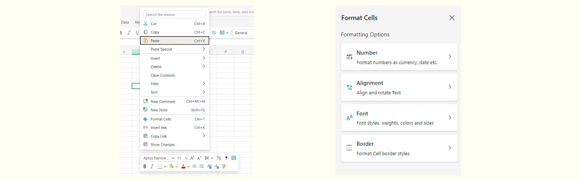
To change the cell format in Excel, you can select a cell or range, then use the shortcut “Ctrl + 1” (the digit one on the keyboard) or right-click and choose “Format Cells”.

The dialog box can also be accessed from “Number > Format Cells” on the “Home” tab. In the “Format Cells” window that appears, you’ll be taken to the “Number” tab, where you can select the desired format. Upon selection, additional format settings for each format type will be displayed beneath the list.

The combination of “Ctrl + Shift” keys along with a key from “`” (tilde) to “6” on the keyboard allows for quick setting of display formats. The formats correspond to the following keys:

“`” (Tilde) – General
“1” – Number
“2” – Time
“3” – Date
“4” – Currency
“5” – Percentage
“6” – Scientific (Exponential)

However, when setting the format using keyboard shortcuts, it is still necessary to open the Format Cells window to edit additional settings. After applying the format, the data in the cell will be displayed according to the selected style.

The “Format Cells” window contains other aspects of visualization, which are located in tabs:

Alignment
Font
Border
Fill
Protection

Applying the correct cell format can enhance data readability and facilitate analysis.

Cell Comments

Comments in Microsoft Excel are textual messages that can be attached to a cell. They are used to explain the content of the cell, provide additional information, or leave notes for other users. Using comments in Excel is beneficial when collaborating on a spreadsheet or creating documents where it’s important to provide additional explanations for cell content.

Adding a comment can be done in several ways:

Select the cell you want to add a comment to and press “Shift + F2”.

Use the context menu key (next to the right Alt key) or “Shift + F10” on the selected cell and choose “Insert Comment” from the context menu.

From the “Review” tab in the ribbon, use the “New Comment” command.

A comment entry box will open, with the system name of the user leaving the comment already filled in. Type your comment text and save it by clicking the “Ok” button.

Viewing Comments

A cell containing a comment is marked with a small triangle in the upper right corner. When a cell with a comment is focused by NVDA, it will announce “Contains comment” between the cell content and its coordinates.

To have NVDA read the content of the comment, use the shortcut “NVDA + Alt + C”. With JAWS, between the content and coordinates of the cell, it will say “Contains comment note”. To have the JAWS screen reader read the content of the comment, use the shortcut “Alt + Shift + ‘ (Apostrophe)”.

JAWS can also display all cells with comments by pressing “Ctrl + Shift + ‘ (Apostrophe)”, and pressing “Enter” on a cell from the list will move the cursor to that cell on the sheet. If you use “Alt + Shift + ‘ (Apostrophe)” on a cell with a comment, JAWS will display the content of the comment in a separate window.

Editing a Comment

Select the cell containing the comment and press “Shift + F2”.

Use the context menu key or “Shift + F10” on the cell and choose “Edit Comment”.

On the “Review” tab in the ribbon, use the “Comment > Edit Comment” command.

A window will open, similar to when creating a comment. Make changes and save them by clicking “Ok”.

Deleting a Comment

Use the context menu key or “Shift + F10” on the cell and choose “Delete Comment”.
On the “Review” tab in the ribbon, use the “Comment > Delete” command.

The “Review” tab contains various tools for working with comments.

Note: It’s important to remember that comments are not displayed in printouts and do not affect cell values. They simply provide additional information for the user.